Assignment 4

The data come from an experiment in which extracellular potentials were recorded from an electrode inserted in layer 5 of primary motor cortex, during a visually guided arm reaching task (Scott et al., 2001, Gribble & Scott, 2002).

The task was to move the hand from a central start target to one of 8 peripheral targets spaced around the circumference of a circle (importantly the spacing was not equal). Each target was presented in random order, and movements to each of the 8 targets were repeated 5 times.

For each movement to each target, two quantities were computed:

1. the mean number of spikes per second over a window starting 150 ms before movement onset (as defined by the acceleration of the hand) and ending at peak hand velocity, and
2. the movement direction (in radians) of the hand at peak acceleration

Here we will consider data recorded from 100 neurons. For each neuron we have two files — one file contains the movement direction data and a second file contains the neural firing data. For example, for neuron 001 we have:

cell_dirs_001.txt

8.4748542e-01   1.1952706e+00   1.7959900e+00   3.2095020e+00   4.2338855e+00   4.7988962e+00   5.4260935e+00   5.7792185e+00
8.8519623e-01   1.1456351e+00   1.8273681e+00   3.2718287e+00   4.1625064e+00   4.6994474e+00   5.5492588e+00   5.9753649e+00
8.4209505e-01   1.2769631e+00   1.6570527e+00   3.2343219e+00   4.3258268e+00   4.7441638e+00   5.5040137e+00   5.9171973e+00
7.4938015e-01   1.1950453e+00   1.5838486e+00   3.1628027e+00   4.2176710e+00   4.6306195e+00   5.4205861e+00   5.7437683e+00
8.0512714e-01   1.2494470e+00   1.7365013e+00   3.2258285e+00   4.2583196e+00   4.7343349e+00   5.3612792e+00   5.8834072e+00

cell_spks_001.txt

1.0000000e-12   2.6315789e+00   2.2471910e+00   5.2747253e+01   6.9662921e+01   5.2500000e+01   3.7362637e+01   2.6262626e+01
2.8169014e+00   2.5316456e+00   6.5217391e+00   4.1304348e+01   6.1728395e+01   6.2068966e+01   3.3684211e+01   1.9801980e+01
5.4054054e+00   1.0000000e-12   1.0000000e-12   2.8235294e+01   7.4074074e+01   5.5172414e+01   3.3663366e+01   2.2448980e+01
5.2631579e+00   1.0000000e-12   2.4096386e+00   3.5555556e+01   7.7272727e+01   7.3563218e+01   3.7254902e+01   1.6494845e+01
4.9382716e+00   2.5974026e+00   4.7619048e+00   4.5360825e+01   7.6923077e+01   7.1604938e+01   3.4042553e+01   1.9417476e+01

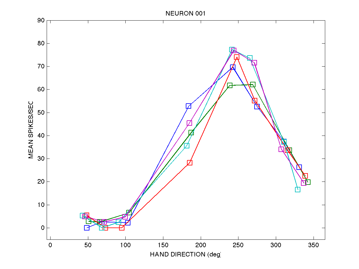
For neuron 001 we have 5 movements (rows) to each of 8 targets (columns). The file cell_dirs_001.txt contains the direction of hand movement (in radians) for each of the 20 movements, and the file cell_spks_001.txt contains the mean activity (spikes per second) over a window beginning 150 ms before movement onset and ending at peak hand velocity.

Here is a graphical depiction of the data for neuron 001:

Here is some sample MATLAB code to load in cell 001, plot the data, and compute the preferred directions of each of the 5 trials: code/plate_sample_code.m.

The goal here is to compute the preferred direction of each neuron — that is, the direction of movement for which the neuron fires most enthusiastically (most spikes per second) — and to conduct a statistical test of whether each neuron is in fact directionally tuned.

The ultimate goal is to look at the distribution of preferred directions across the population of directionally tuned neurons to see if all movement directions are equally represented.

Computing the preferred direction of a neuron is relatively easy, in cases where the movement directions are spaced equally around the unit circle. In the so-called vector method, all we have to do is sum together individual vectors whose directions represent the directions of movements and magnitudes (vector lengths) represent the spiking rate in those directions. The direction of the resulting vector sum will represent the preferred direction of the neuron. See Georgeopoulos et al., 1986 & 1988 for an example:

Georgopoulos, A. P., Schwartz, A. B., & Kettner, R. E. (1986). Neuronal population coding of movement direction. Science, 233(4771), 1416-1419.

Georgopoulos, A. P., Kettner, R. E., & Schwartz, A. B. (1988). Primate motor cortex and free arm movements to visual targets in three-dimensional space. II. Coding of the direction of movement by a neuronal population. The Journal of Neuroscience, 8(8), 2928-2937.

In our case however we do not have movement directions that are spaced equally around a unit circle. Taking the simple vector sum will result in biases. There are a number of possible solutions to this problem (see Gribble & Scott 2002).

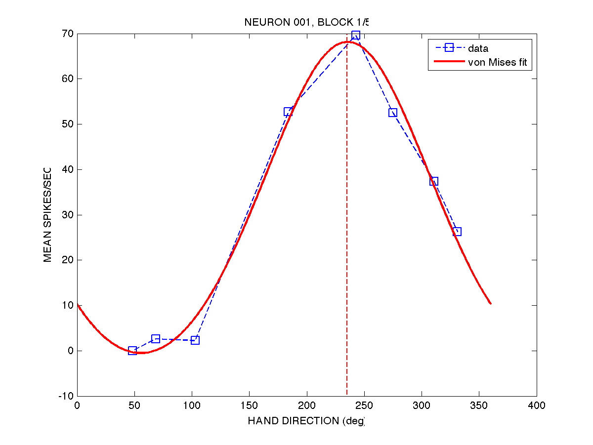
One solution is to fit the unequally-spaced data to a function (such as a cosine function, or a von Mises function), and then determine the movement direction corresponding to the peak of that function. See Equations 30 and 31 in Gribble & Scott 2002 for cosine and von Mises functions. Here is an example of fitting a von Mises function to the first 8-target movement set for neuron 001. We can then simply pick off the hand direction corresponding to the peak, to get the preferred direction of the neuron.

The weaknesses of this approach is that fitting functions (e.g. using optimization techniques) can be time consuming since optimization is an inherently iterative procedure, and sometimes the fit may not converge on a global minimum. On ther other hand, computers are fast now and we have strategies to deal with local minima (e.g. re-running the optimizations many times from different initial guesses).

Another solution to the problem of non-uniformly spaced directions was proposed in Gribble & Scott 2002, that involves a series of direct calculations (the so-called plate method). The advantage of this method is that there is no iterative optimization, and so it is faster, and what's more there is no danger of non-convergence.

For this assignment I will provide a function called platemethod() that will compute the preferred direction of a neuron given an array of directions and an array of spike counts. You are welcome to use it in your assignment. If you would prefer to use an optimization approach for your assignment, by all means go ahead and do that. You have the knowledge and the tools now to do it.

Here is a gzipped tarred directory containing platmethod functions in MATLAB, in Python, in R and in C:

• platemethodfuns.tgz

For each neuron we have 5 repetitions of 8-target movements. To estimate the PD for each neuron we can take the mean PD for each of the 5 8-target repetitions. Be careful though, taking the mean of angles is not always straightforward. For example, what is the mean of 2 degrees and 358 degrees? If you simply take the arithmetic mean you get ((2+358)/2) = 180 degrees. In fact what you want is 0 deg (or equivalently, 360 deg). The problem is angles "wrap around" 360 deg.

There is a branch of statistics that has been developed to adapt common measures and methods to angular data, called circular statistics. For example, see this Wikipedia page for a discussion of how to compute the mean of circular quantities. There are several books on circular statistics including:

Batschelet, E., Batschelet, E., Batschelet, E., & Batschelet, E. (1981). Circular statistics in biology (Vol. 371). London: Academic Press. Chicago

Another way to estimate the PD of the neuron from all the data is to just consider the (5 x 8) data set as a single set of data with 40 movements, and run that throught the plate method (or through your optimizer if you're fitting it to a function). I will leave it up to you to decide how to estimate the mean PD.

You can imagine that for a neuron that is not directionally tuned, if you nevertheless compute a preferred direction for it, and you do this multiple times, with a different set of movements each time, what will happen is that each time you compute a preferred direction, it will be different than the last one … and over many repetitions, you will get preferred directions all over the place (they will not be very consistent). On the other hand if a neuron is highly tuned, then each time you compute a preferred direction, the result will be consistent from movement set to movement set.

To quantitatively test whether a neuron is tuned, we can do the following, as long as we have multiple 8-target movement sets for the neuron (we do in this case, we have 5 repetitions for each target direction).

1. for each of the 5 8-target movement sets \(i\), compute the preferred direction \(pd_{i}\) of the neuron
2. construct a vector \(v_{i}\) whose length is \(1\) and whose direction is the preferred direction computed from each 8-movement set \(pd_{i}\)
3. add the 5 vectors \(v_{i}\) together (vector addition) and compute the length \(r\) of the resulting vector.

The logic is, the more consistent the \(pd\) is over repetitions of the 8-movement target set, the larger \(r\) will be.

Now that we have a measure of directional tuning (\(r\)), we can do a statistical test to determine whether \(r\) is "significant" or not. The way we will do this is by using a bootstrapping or resampling technique. Here is what we will do.

We will repeat the following procedure a large number of times (e.g. 10,000):

1. Create a new set of (5 x 8) spike data, by randomly sampling, with replacement, from the original set.
2. Compute \(r\), the measure of tuning
3. Save \(r\) to a list (of 10,000 \(r\) values over the 10,000 repetitions of this procedure)
4. Once we have our 10,000 \(r\) values, determine what proportion of the 10,000 simulated \(r\) values are as large or larger than the empirically observed r value, which we computed above.

The logic here is that in our 10,000 simulations, we are simulating the null hypothesis where the null hypothesis is that the neuron is not directionally tuned, and the spike count for a given direction is random (in this case, randomly sampled from the "population" of (5 x 8) spike counts collected for each neuron). If the actual \(r\) value we compute based on the actual data is less than 5% likely in our simulation of the null hypothesis, we reject the null hypothesis that the neuron is not directionally tuned, and we conclude that it is in fact directionally tuned.

For example, if we take neuron 005, I have computed using the plate method that the measure \(r\) of direction tuning is \(r=3.9804\). When I perform a bootstrap test using 10,000 iterations, I get the following distribution of \(r\) values under the null hypothesis (i.e. when I randomly sample with replacement from the original (5 x 8) set of spike data:

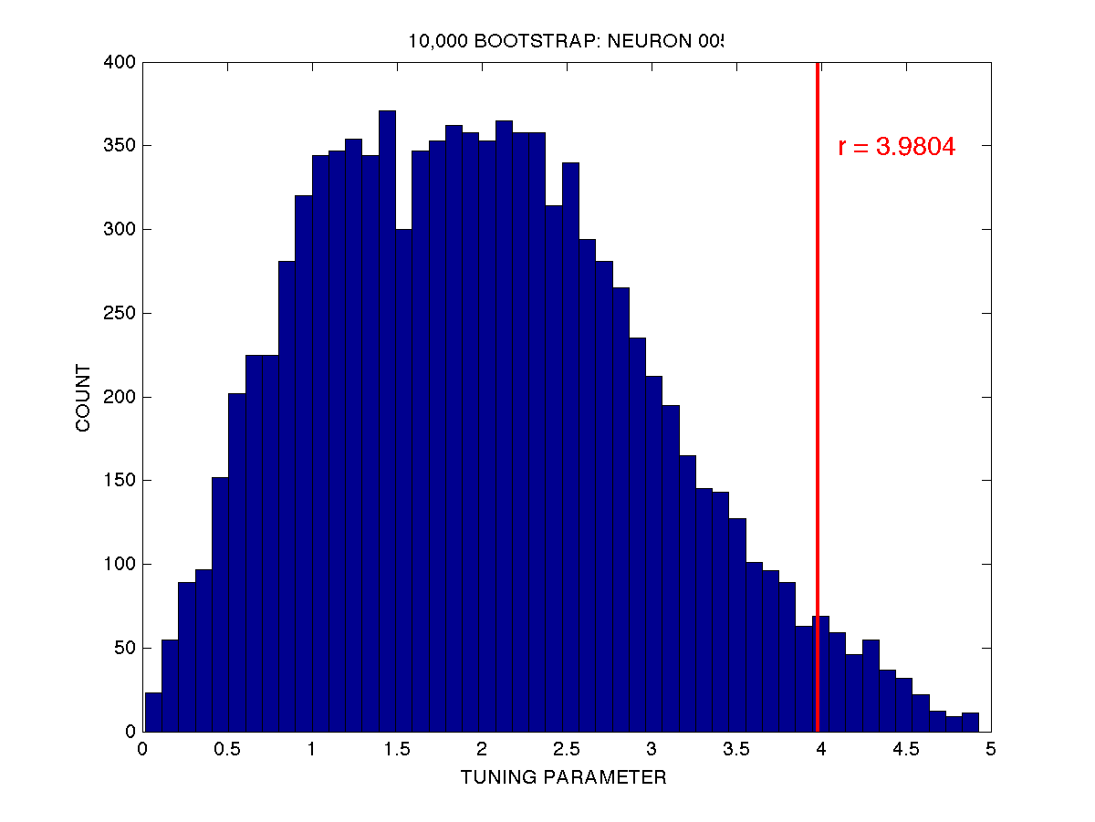
The observed tuning parameter \(r\) is plotted as a vertical red line overtop of the distribution of \(r\) under the null hypothesis, as assessed by the bootstrap test using 10,000 random resamplings (with replacement) of the spike data. As you can see only a small proportion of the bootstrap values of \(r\) are greater than our observed value of \(r=3.9804\). In fact if we count, there are 331 out of 10,000 that are greater than or equal to \(r=3.9804\). This corresponds to \(p = 0.0331\). If we use an alpha value of \(p = 0.05\) as our cutoff for rejecting the null hypothesis, we would indeed reject the null in this case (the null being that the neuron is not directionally tuned) and we would conclude that the neuron is in fact directionally tuned. Actually if we want to be technically correct from a statistical point of view, we would say that the chances are very low that the cell is not directionally tuned… i.e. assuming the null hypothesis is true, the chance of observing a tuning parameter \(r\) as extreme or more extreme than the one we actually observed is only 3.31 %. If we wanted to be more conservative we could set our alpha level at \(p = 0.01\).

When testing your code, perhaps set the number of bootstrap iterations to 1,000 or even 100 for testing pruposes. When you are confident your code is working, set it to 10,000 and go get a coffee.

So your tasks are:

1. Compute an estimate of the preferred direction of each neuron.
2. Count how many neurons out of 100 are directionally tuned (using whatever alpha level cutoff you wish)
3. For those neurons that are directionally tuned, graphically display the distribution of preferred directions over the population of neurons.

Submit items 1. 2. and 3. above as a short (1 page max) report (pdf format please).

1. create a file called PD.txt that contains the preferred direction (in radians, to 8 decimal places) for each of the 100 neurons. The file should be 100 lines long (1 line per neuron).
2. create a file called PDboot.txt that contains the bootstrap probability (to 8 decimal places) for each of the 100 neurons. The file should be 100 lines long (1 line per neuron).

Send me: (by email):

• your 1-page .pdf report
• the PD.txt file
• the PDboot.txt file
• your code

I should be able to run your code on my machine and it should generate the PD.txt file and the PDboot.txt file. You can assume that I will run your code from a location that contains the neurondata/ subdirectory.

When I run my code with 10,000 bootstraps on the 100 neurons, here is what I get in terms of neurons that are significantly tuned:

• p < .050 : 92 neurons
• p < .010 : 78 neurons
• p < .005 : 73 neurons

You may not get the exact same numbers as me, since your random selection in your bootstrap will be different … but you ought to get something relatively close.

For p < .05, the neurons that are not significantly tuned, at least in my code, are neurons:

41, 42, 43, 55, 56, 66, 76, 85

If anyone is really struggling, just come and see me, I can help. I'd rather everyone see the assignment through to the end, even if you need some help, than for some to not finish.

As a benchmark, here are the PDs (in radians) of the 5 repetitions for the data from neuron 001, using the supplied platemethod function in MATLAB:

4.0845 4.3150 4.3715 4.3153 4.2462

You should get something pretty much identical in your Python or R version of the platemethod function.

Here is what the first 3 lines of PD.txt look like for my solution (where I take the entire 5x8 dataset for each neuron as a whole and compute PD):

4.29683956
4.16177382
4.26387645

When I compute a neuron's PD as the mean (using circular stats approach) of the 5 PDs for the 5 trials, I get the following mean PDs for the first 3 neurons:

4.26666622
3.97270313
4.37791813

You can compute PD for each neuron using either of these methods, it's up to you.

Finally, time your code: how long does it take to compute the estimate of the preferred direction, and the bootstrap probability, for all 100 neurons, using 10,000 bootstrap iterations? We will have a contest to see whose code runs the fastest (we will run it on my laptop). The winner gets a prize.

The leaderboard will be updated as people submit their code:

speed contest leaderboard

When writing your code, assume the data are located in a subdirectory relative to the location of your code, called neurondata/. You can download the data directory here:

neurondata.tgz

I should be able to put your code in a directory containing neurondata/ and run your code without adjusting anything.